Binary outcome
Predict the purchase decision, not the sale price: 1 indicates purchase and 0 indicates no purchase.
An end-to-end machine learning case study exploring whether a prospective buyer decides to purchase a property. I compared neural network architectures, applied hyperparameter optimization, and rebuilt the evaluation pipeline to distinguish promising model performance from trustworthy generalization.
Buying a house is not just a question of property characteristics. The dataset connects buyer, financial, and property-related variables to a binary decision outcome.
Predict the purchase decision, not the sale price: 1 indicates purchase and 0 indicates no purchase.
Combine numerical and categorical inputs using a consistent preprocessing pipeline suitable for neural networks.
Evaluate generalization with appropriately separated data, class-aware metrics and explicit uncertainty about historical outputs.
Data came from the publicly listed Global House Purchase Decision Dataset on Kaggle. No original records are redistributed from this portfolio or the accompanying repository.
Because fewer than one in four records belong to the positive class, I use precision, recall, F1 and precision–recall AUC alongside accuracy.
The public repository refactors the initial notebook into modules and fixes an important experimental weakness: preprocessing and hyperparameter decisions must not use the final test data.
Load and validate the tabular dataset locally.
Stratified training, validation and final test partitions.
Fit transformations using only the training partition.
Train networks and tune on validation data.
Evaluate the selected model with untouched holdout data.
The repository also includes a logistic regression baseline, automated checks, saved model artifacts, and an optional local Streamlit inference interface.
The study focused on multilayer perceptrons (MLPs) for structured data. The public implementation preserves an original architecture and a historically selected optimized architecture for comparison.
A simpler baseline to check whether additional deep-learning complexity improves predictive performance.
A feed-forward network trained on encoded, scaled tabular features. Its historical learning curves are retained for inspection.
The selected hidden-layer widths from the original experiment, with dropout 0.15 and Adam learning rate approximately 0.001967.
Instead of selecting network settings manually, the project uses Optuna to explore candidate configurations. The revised implementation selects parameters using validation average precision, not final test scores.
The notebooks configured a 20-trial Optuna study. The exported learning curves are available, but a complete auditable trial-history database was not provided.
Important: this earlier workflow reused test data during model selection. Its reported results are historical evidence only.
The GitHub version stores studies locally, keeps validation and test roles separate, and supports reproducible command-line training.
No private Optuna dashboard, DagsHub account, MLflow credentials, or access tokens are required.
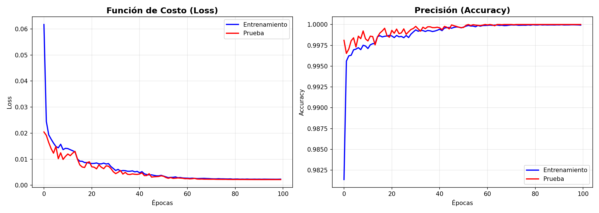
These three figures come from the original notebooks. They illustrate training behavior, but the validation curves must not be interpreted as measurements from an independent untouched test set.
Historical training and validation curves for the neural baseline.
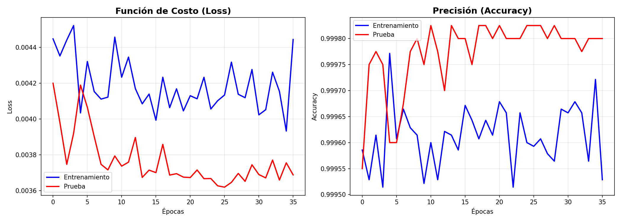
Historical learning curves after selecting a different neural network configuration.
Additional saved training curves from the optimization work.
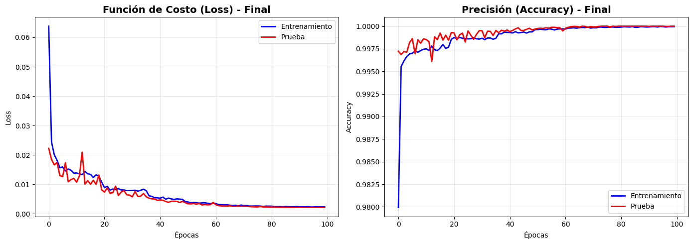
The original notebook reported an optimized confusion matrix without errors on a 40,000-row split. That result is an archived observation, not proof that the system predicts real-world home purchases with perfect accuracy.
Saved notebook outputs showed extremely high prediction scores; the split was involved in model selection, so those scores cannot serve as untouched-test evidence.
The new experiment reserves 20% of data for final testing and tracks precision, recall, F1, balanced accuracy, ROC AUC and average precision.
Ablation studies and testing across different countries or populations could reveal how much the model relies on decision-adjacent variables.
More than optimizing a neural network, this project showed me the difference between a convincing score and a defensible machine learning experiment.
A model is only as credible as its evaluation protocol. Refactoring the original notebook helped turn a one-off experiment into a reproducible ML project with clear evidence, limitations and separation of responsibilities.
I learned why fitting preprocessing on all rows, or repeatedly using test observations for decisions, produces overoptimistic conclusions even when the code runs correctly.
Hyperparameter tuning is useful only when it optimizes a meaningful validation metric. Class imbalance made average precision especially relevant here.
Separating data preparation, model configuration, training, reports and inference makes debugging and comparisons much easier than keeping everything inside notebooks.
Unusually strong results pushed me to question feature shortcuts, dataset design, class imbalance and how predictions could change outside the sample.
My main takeaway was to make every stage of model development auditable: how data is split, which metric selects a model, what the test score actually measures and which conclusions remain unverified.
The public repository contains reproducible scripts, an optional interactive demo, testing utilities and documentation. Original data and all service credentials stay outside source control.
Read the README, run the pipeline, compare model architectures and inspect historical results with their limitations documented.
Explore repository ↗Get the dataset from its original source. No buyer records are embedded in this portfolio webpage.
View dataset ↗